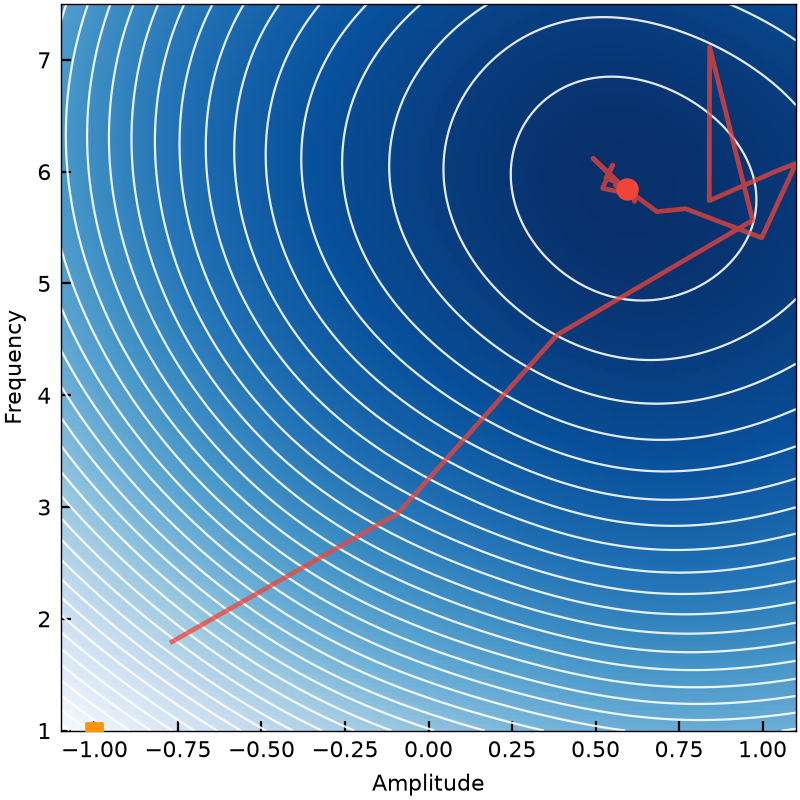
Full-covariance CMA-ES
 PELAGIC SYSTEMS
REAL-TIME CONTROL
Optimization, sampling, estimation, and feedback — directly inside the experiment.
01 / THE REAL-TIME TOOLBOX
Optimization, estimation, machine learning, and more — running directly inside your quantum experiment.
Full-covariance CMA-ES
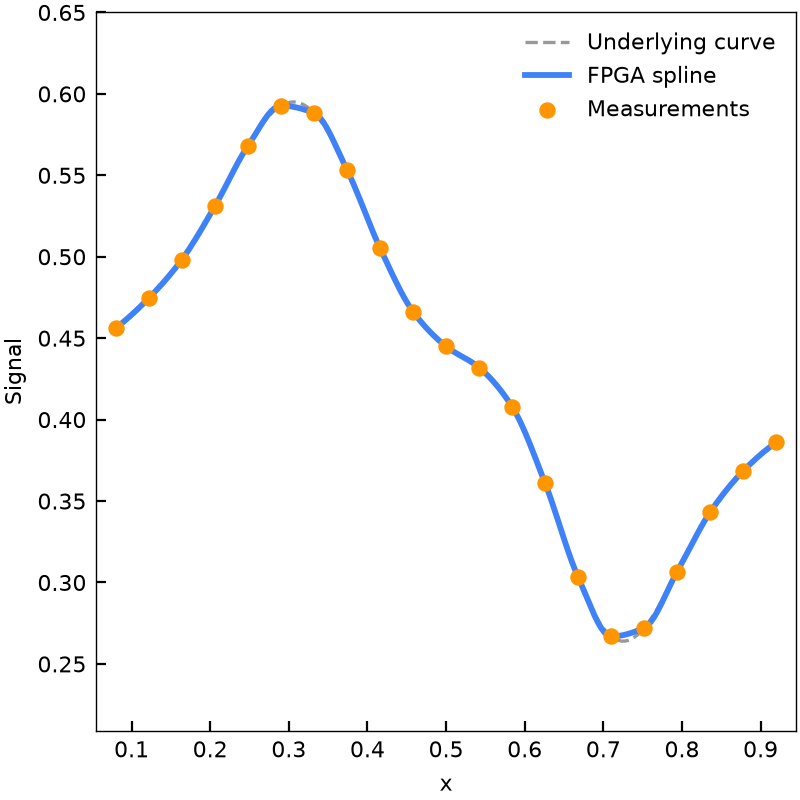
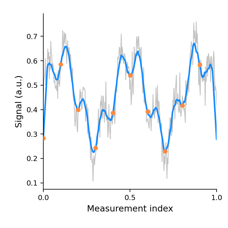
Incremental spline estimation
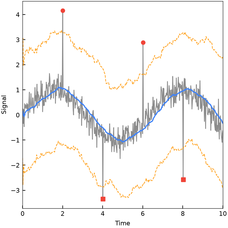
Running z-score event detection
DBSCAN clustering
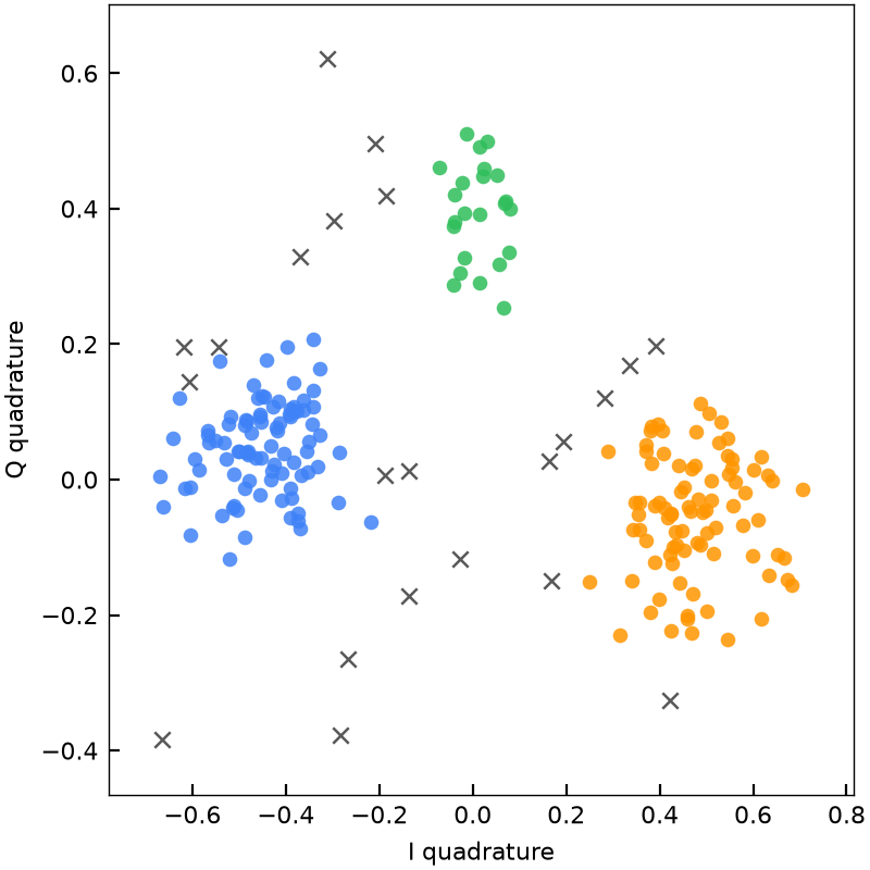
Least-squares matrix solve
Adaptive sampling
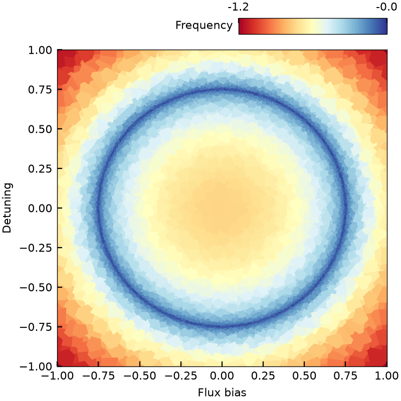
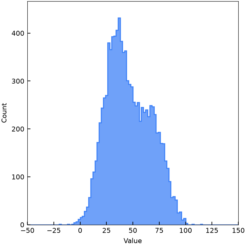
Streaming histogram
Three-point T₁ estimation
02 / FAMILIAR SYNTAX
Take the scientific tools you know into the experiment. Start with a familiar interface.
from scipy.signal import find_peaks

peaks, prop = find_peaks(signal, height=0.0, distance=50)
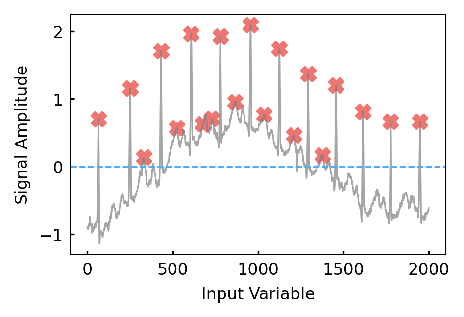
from pelagic.fpga.signal import find_peaks

peaks, prop = find_peaks(signal, height=0.0, distance=50)
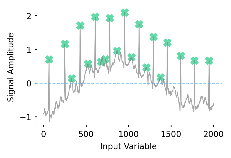
The same peak-finding call, with only the import changed.
03 / FULL EXAMPLE
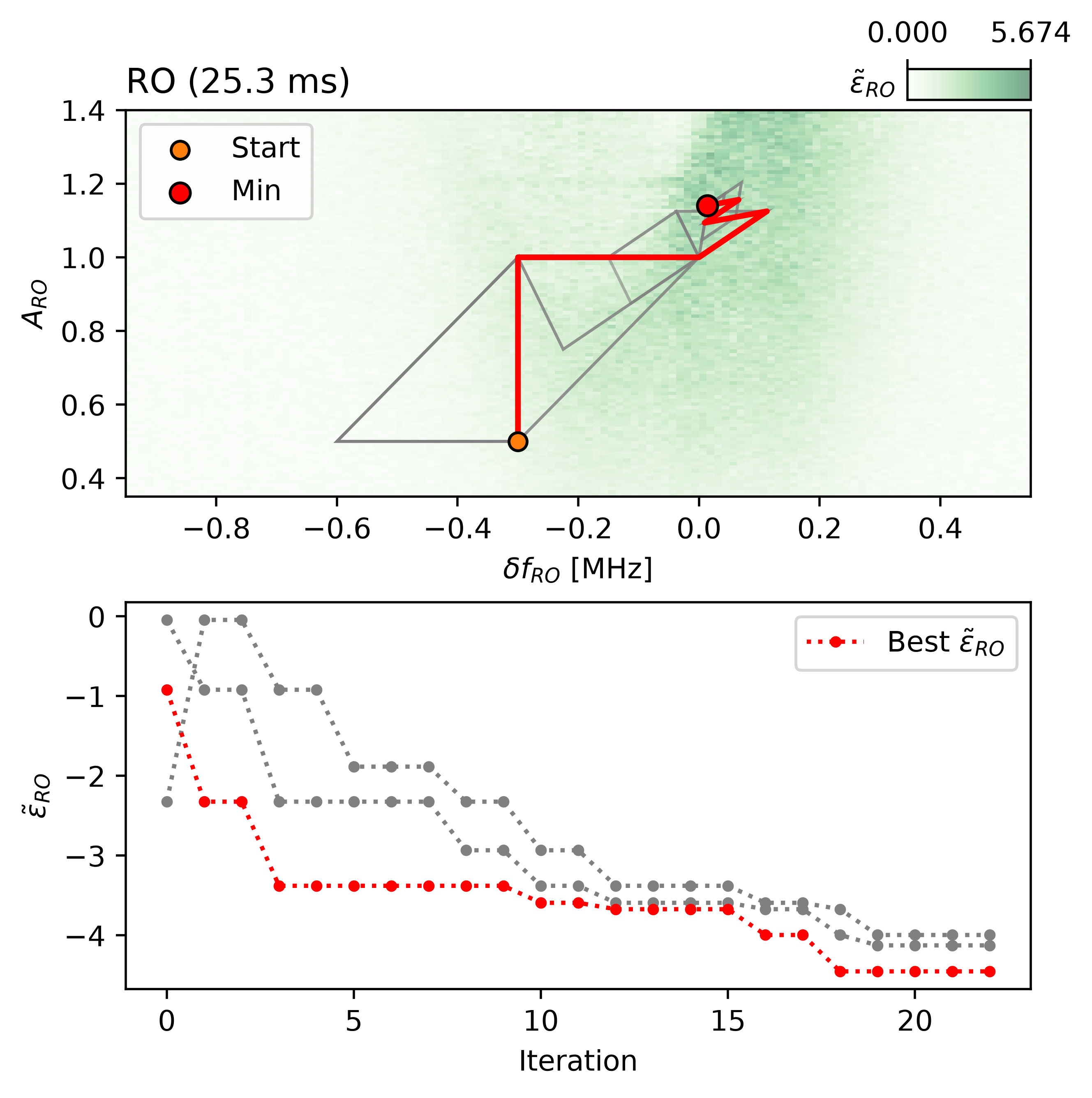
Minimize readout error with Nelder–Mead. Each measurement guides the next frequency offset and amplitude, tracing a path toward an optimized operating point.
from pelagic.fpga.optimize import minimize

def objective(parameters):
    frequency_offset, amplitude = parameters
    # Experiment-specific readout-error acquisition.
    return measure_readout_error(frequency_offset, amplitude)

# x0: (frequency offset, amplitude).
result = minimize(
    objective,
    x0=initial_readout_parameters,
    method="Nelder-Mead",
)
04 / RETHINK THE EXPERIMENT
When analysis can happen inside the experiment, the experiment itself can change. Design around what you learn, instead of a fixed list of measurements.
Use the response you just measured to decide where to probe next, rather than committing to an entire sweep in advance.
Make your stopping rule part of the experiment. Continue collecting information where uncertainty matters.
Estimate a parameter, change a delay, or select a new branch inside the same control sequence.
05 / CLOSE THE LOOP
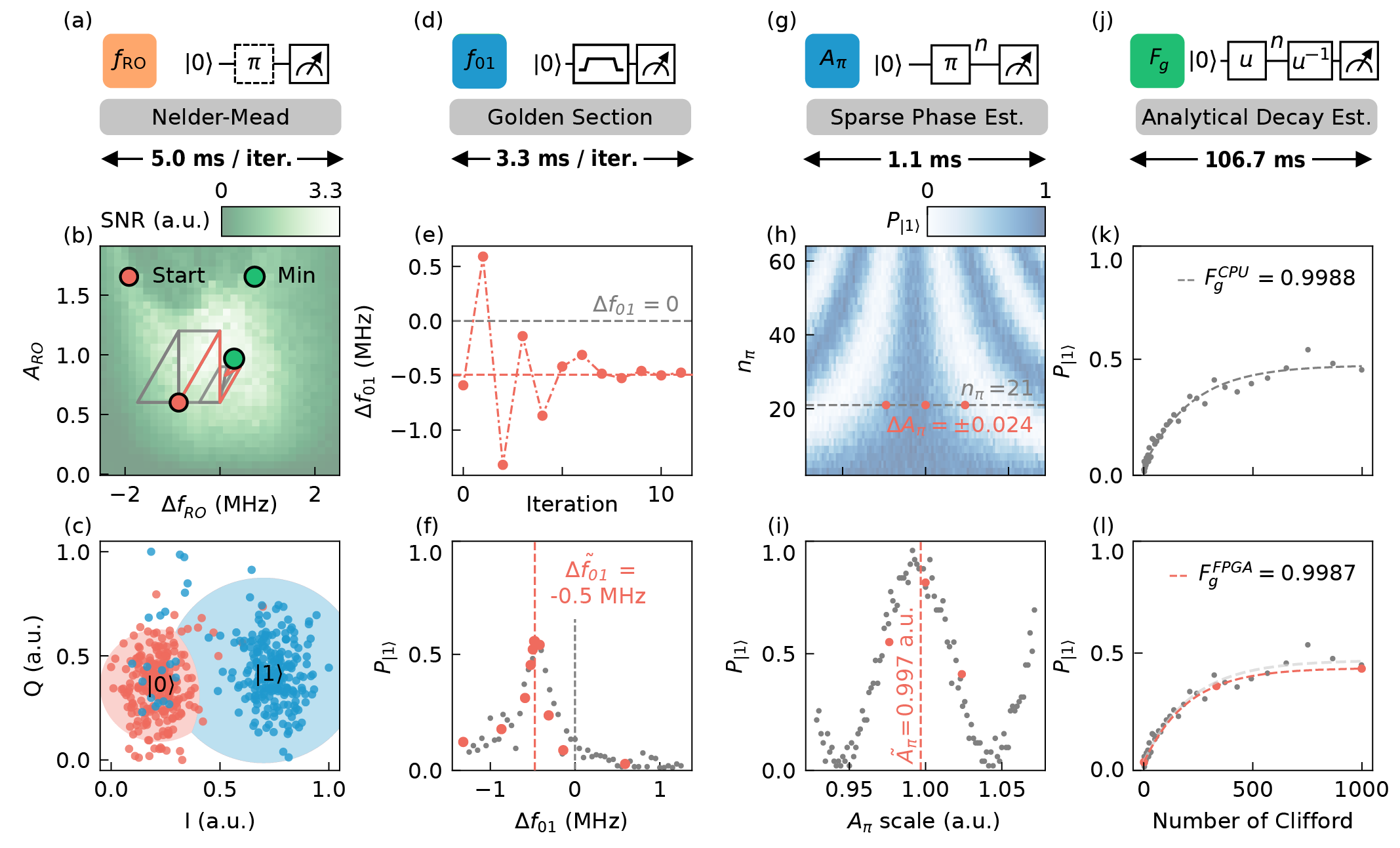
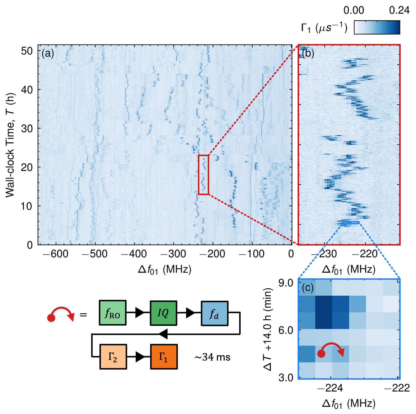
Combine five real-time calibration experiments into one on-FPGA workflow. Keeping readout, drive, and coherence measurements together lets you explore a changing quantum device on its own timescale.
~34 msper complete five-stage cycle
Running on FPGAOptimize the readout setting.
Set the state-discrimination boundary.
Track the qubit resonance.
Estimate the loss of coherence.
Estimate energy relaxation.
Approximately 34 ms for the illustrated five-stage cycle, not the entire frequency sweep.
Repeat the combined workflow across qubit frequency and over time to resolve two-level-system (TLS) dynamics. The measured relaxation-rate map below reveals how loss features move and fluctuate while the device is recalibrated.
stm = StreamManager()
axt = stm.axis_tracker

with program() as prog:
    i, flux = declare(int), declare(fixed)  # Iteration, flux point.

    with axt.add_axis(for_(i, 0, i < n_iterations, i + 1), name="iteration"):
        # (1) Reset initial parameters.
        set_initial_parameters(qubit)

        with axt.add_axis(for_each_(flux, flux_points), name="flux_point", unit="V"):
            # (2) Set flux point.
            qubit.z.set_dc_offset(flux)

            # (3) Calibrate the qubit at the flux point.
            qubit.calibrate_readout_frequency(stm=stm, apply_correction=True)
            qubit.calibrate_iq_threshold(stm=stm, apply_correction=True)
            qubit.calibrate_drive_frequency(stm=stm, apply_correction=True)

            # (4) Estimate decoherence times.
            qubit.estimate_t2_echo(stm=stm)
            qubit.estimate_t1(stm=stm)

    with stream_processing():
        stm.process()  # Automatically reshape data into an xarray.Dataset.
06 / PROVEN ON QUANTUM HARDWARE
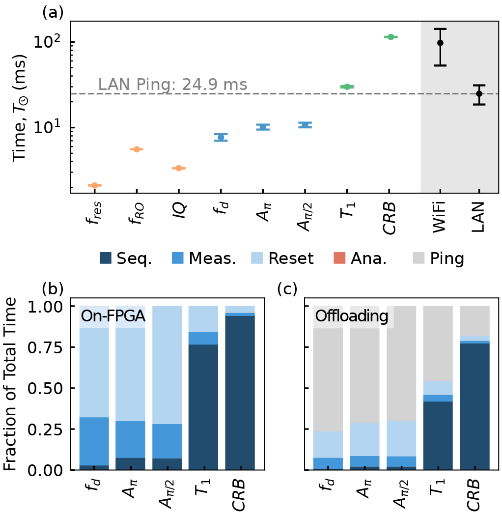
On-FPGA acquisition and analysis keep calibration decisions close to the experiment. Demonstrated on a superconducting quantum processor.
From the first experimental shot to an estimate available on the controller.
Reported T₁ resultPulse execution, acquisition, and reset dominate the reported timing budget.
PELAGIC REAL-TIME
Bring your next experiment into the control loop. Let’s talk about what you want to measure, learn, and change.