SCIENTIFIC FOUNDATIONS

Every measurement
has a story.

A measurement is more than a number. It has units, uncertainties, coordinates, and a history. Pelagic keeps them connected, from the first pulse to the final result.

Explore the foundations

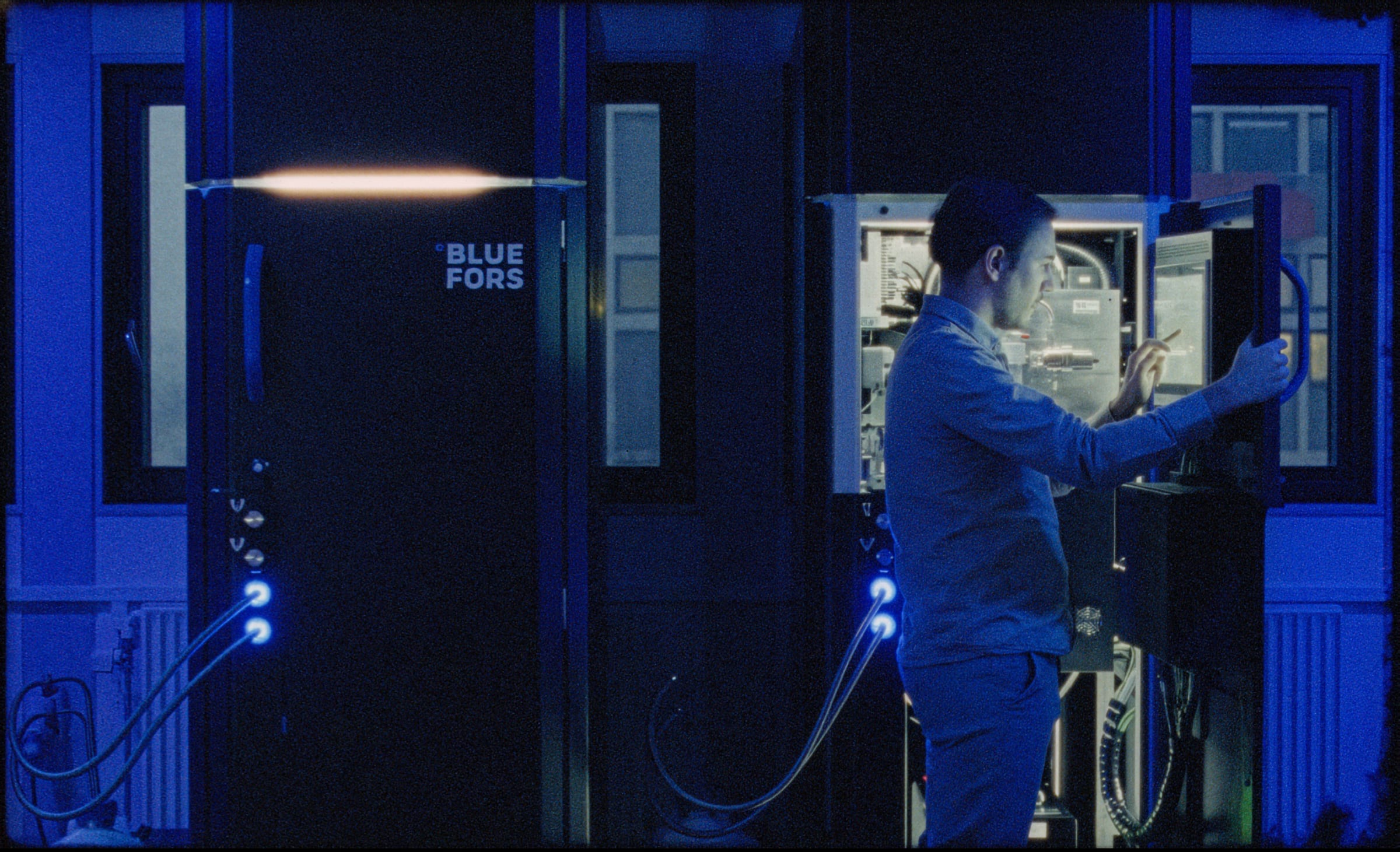
A researcher working with a quantum experiment in the laboratory.

01 / SCIENTIFIC QUANTITIES

A number is never
just a number.

Pelagic treats physical units and uncertainties as part of the calculation, not annotations added afterward. Physical meaning stays with the data, through every step of the analysis.

01 / UNITS

Units follow the calculation.

Multiply or divide quantities inside an xarray Dataset. Their units follow the operation, and compact_units presents the result at a useful scale.

Voltage

200\,\mathrm{mV}

Current

400\,\mu\mathrm{A}

Multiply · power

V\times I=80\,\mu\mathrm{W}

Voltage × current

Divide · resistance

V/I=500\,\Omega

Voltage ÷ current

u.compact_units(ds)Readable scales. Physical meaning intact.

Units in an xarray Dataset

PYTHON

ds["power"] = ds.voltage * ds.current
ds["resistance"] = ds.voltage / ds.current
ds = u.compact_units(ds)

Illustrative electrical quantities. Units are attached to the input variables in the Dataset.

02 / ERROR PROPAGATION

Uncertainty follows the transformation.

Convert a complex IQ signal to its magnitude and carry its uncertainty with it. The uncertainty in I and Q projects onto the radial direction, including their correlation.

z=I+iQ\quad\longrightarrow\quad |z|=\sqrt{I^2+Q^2}

z = I + iQabs(z)

Magnitude · propagated uncertainty

|z|=(0.400\pm0.026)\,\mathrm{mV}

Illustrative IQ estimates. The ellipse shows joint 1σ uncertainty; the magnitude error uses first-order propagation of the full I/Q covariance.

How the uncertainty is propagated

\sigma_{|z|}^2=\frac{I^2\sigma_I^2+Q^2\sigma_Q^2+2IQ\,\operatorname{Cov}(I,Q)}{I^2+Q^2}

The I/Q example uses the full covariance and a first-order approximation. The points visualize the joint uncertainty of the complex estimate.

02 / SCIENTIFIC DATASETS

Your data should know
what it represents.

An array of numbers is useful. An array with named dimensions, physical coordinates, and experimental context is something you can build science on.

BUILT ON XARRAY

xarray.Dataset5 qubits · 13 amplitudes · 161 frequencies

DATA VARIABLES

excited_population(qubit, drive_amplitude, drive_frequency)

standard_error(qubit, drive_amplitude, drive_frequency)

COORDINATES

drive_frequency1615.15 … 5.31 GHz

drive_amplitude130.05 … 0.35 V

qubit5q1 · q2 · q3 · q4 · q5

SELECT A SLICEq1 · drive_amplitude = 0.20 VOne spectrum. Its coordinates intact.

q1 · drive_amplitude = 0.20 V

One named slice from the illustrative dataset.

<xarray.Dataset>
Dimensions: (qubit: 5, drive_amplitude: 13, drive_frequency: 161)
Coordinates:
  qubit             q1  q2  q3  q4  q5
  drive_amplitude   [V] 0.05 … 0.35
  drive_frequency   [GHz] 5.15 … 5.31
Data variables:
  excited_population   (qubit, drive_amplitude, drive_frequency)
  standard_error       (qubit, drive_amplitude, drive_frequency)
Attributes: experiment=Qubit spectroscopy; run=0042; shots_per_point=1000; source=synthetic

Data variables share named dimensions and coordinate arrays. This illustrative dataset contains five qubits, a drive-amplitude sweep, and a frequency axis; the selected spectrum is q1 at 0.20 V.

03 / SCIENTIFIC MODELS

Fit the physics.
Not the framework.

Fit a single model, compose it with other physical components, or apply it along a named axis. The same analysis can follow your data from one trace to a complete scan.

COMPOSABLE MODELS · EXTENDED IMINUIT

01
Fit a model
Describe one physical response.
02
Compose models
Combine resonances and a background.
03
Follow an axis
Fit every slice without reshaping your data.

The measurement Illustrative data

The fitted model Fit along drive_frequency

Illustrative data and actual offline fits, on the same color scale. Each amplitude slice is fitted independently along drive_frequency; the right-hand image is evaluated from those saved fit parameters.

Inside one spectrum · q1 at 0.20 V

Explore the componentsResonance 1Resonance 2BackgroundTotal model

Illustrative model, fitted offline. Toggle components to explore their sum; observations and the stored full-model result stay fixed. No optimizer runs in the browser.

Fit · compose · apply along an axis

PYTHON

model = (
    Lorentzian()
    + Lorentzian()
    + Background()
)

# One trace
result = model.fit(spectrum)

# Every amplitude, along the frequency axis
results = model.fit(
    data, axis="drive_frequency"
)

Illustrative pseudocode, not a verified Pelagic SDK API. The example data were fitted offline with SciPy; the website displays the saved result.

STORED FULL-MODEL RESULT

f_{01}=(5.233818\pm0.000084)\,\mathrm{GHz}

Run 0042 · approximate 1σ · reduced χ² = 0.96

04 / REPRODUCIBILITY

Come back tomorrow.
Or in six months.

Revisit measurements. Improve models. Compare calibrations. See what changed between runs, and understand how a result was produced.

COMPARE RUNS · REVISIT RESULTS

EXAMPLE RUN003920 Apr 20265.230860 GHz
EXAMPLE RUN004020 Jun 20265.231767 GHz
EXAMPLE RUN004120 Aug 20265.232868 GHz
LATEST EXAMPLE004220 Oct 20265.233818 GHz

WHAT CHANGED

Run 0039 0042

Analysis revision: example-1; example-4
Readout amplitude: 0.12 V; 0.15 V
Pulse duration: 40 ns; 48 ns
Fitted frequency: 5.230860 GHz; 5.233818 GHz

● Run 0039● Run 0042

Illustrative dates, settings, and measurements. Highlighted differences do not establish that configuration changes caused the observed frequency shift.

05 / THE BIG PICTURE

The physics changes.
The context stays.

Units stay consistent. Uncertainties propagate. Data remains structured. Models stay reusable. Results retain their history.

NOTHING IMPORTANT GETS LEFT BEHIND.

Quantities
Dataset
Model
Saved result

ONE EXPERIMENT · ITS CONTEXT INTACT

q1 · Qubit spectroscopy · Run 0042 · Illustrative data

f_{01}=(5.233818\pm0.000084)\,\mathrm{GHz}

SCIENTIFIC FOUNDATIONS

Your experiments
deserve a memory.

Good science depends on more than good measurements. It depends on knowing what was measured, how it was analyzed, and what changed along the way. Pelagic brings those foundations together, so you can focus on understanding the physics.

Explore the Experiment Framework Talk to Pelagic

Every measurementhas a story.

A number is neverjust a number.

Units follow the calculation.

Uncertainty follows the transformation.

Your data should knowwhat it represents.

Fit the physics.Not the framework.

Fit a model

Compose models

Follow an axis

Come back tomorrow.Or in six months.